LobsteR - Analysing a Decade of High-Frequency Trading

Downloading and extracting massive data

First, I requested all orderbook messages from Lobster up to level 10 from June 2007 until March 2020. During that period, SPY trading was very active: I observe more than 4.26 billion messages. Total trading volume of SPY on NASDAQ during that period exceeded 5.35 Trillion USD.

Lobster compiles the data on request and provides downloadable .7z files after processing the messages. To download everything (on a Linux machine), it is advisable to make use of wget (you’ll have to replace username, password and user_id with your own credentials):

wget -bqc -P lobster_raw ftp://username:password@lobsterdata.com/user_id/*

As a next step, extract the .7z files before working with the individual files - although it is possible to read in the files from within the zipped folder, I made the experience that this can cause problems when done in parallel.

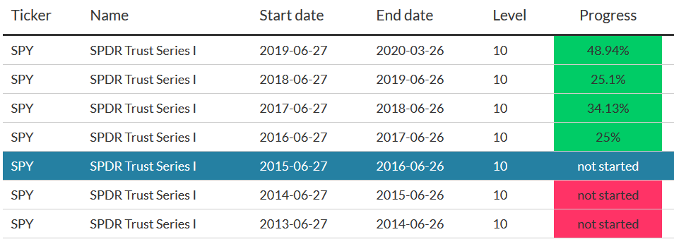
7z e .lobster_raw/SPY_2019-06-27_2020-03-26_10.7z -o./data/lobster
7z e .lobster_raw/SPY_2018-06-27_2019-06-26_10.7z -o./data/lobster
7z e .lobster_raw/SPY_2017-06-27_2018-06-26_10.7z -o./data/lobster
....

3208 trading days occupy roughly 3.2 Terabyte of hard drive space. As explained in my previous post, I compute summary statistics for each single day in my sample. For the sake of brevity, the code snippet below is everything needed to do this in a straightforward parallel fashion using Slurm Workload Manager (the actual task 01_summarise_lobster_messages.R can be downloaded here).

#$ -N lobster_summary
#$ -t 1:3208
#$ -e SPY_Investigation/Chunk
#$ -o SPY_Investigation/Chunk
R-g --vanilla < SPY_Investigation/01_summarise_lobster_messages.R

Merge and summarise

Next, I merge and evaluate the resulting files.

# Required packages
library(tidyverse)
library(lubridate)

# Asset and Date information
asset <- "SPY"
existing_files <- dir(pattern=paste0("LOBSTER_", asset, ".*_summary.csv"), 
                      path="output/summary_files",
                      full.names = TRUE)

summary_data <- map(existing_files, function(x)
  {read_csv(x, 
            col_names = TRUE, 
            cols(ts_minute = col_datetime(format = ""),
                 midquote = col_double(),
                 spread = col_double(),
                 volume = col_double(),
                 hidden_volume = col_double(),
                 depth_bid = col_double(),
                 depth_ask = col_double(),
                 depth_bid_5 = col_double(),
                 depth_ask_5 = col_double(),
                 messages = col_double()))})
summary_data <- summary_data %>% bind_rows()

write_csv(summary_data, paste0("output/LOBSTER_",asset,"_summary.csv"))

SPY Depth is at an all-time low

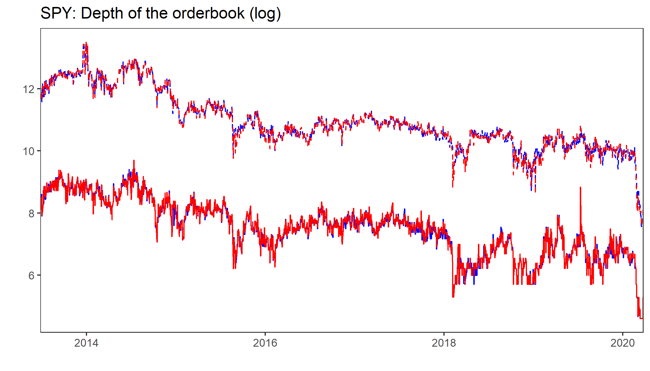
In their paper Bid Price Dispersion, Albert Menkveld and Boyan Jovanovic document (among many other interesting things) a striking downwards trend in depth of the orderbook of SPY, the most actively traded ETF in the world.

data_by_date <- data %>% 
  mutate (date = ymd(floor_date(ts_minute, "day"))) %>%
  group_by(date) %>% 
  select(-ts_minute) %>% 
  summarise_all(median)

Feel free to play around with the Shiny Gadget at the beginning of the post to convince yourself: We see a negative trend in quoted spreads (apart from a couple of outliers) but as the figure below simultaneously shows, quoted depth at the best level as well as 5 basis points apart from the concurrent midquote decreased as well - note the extreme drop in liquidity provisioning since the beginning of 2020. The red line in the figure shows the daily average number of shares at the best ask (blue line corresponds to the bid). The dashed lines correspond to depth at 5 basis points (the number of shares available within 5 basis points from the midquote). Note that the y-axis is in a log scale, thus the figure hints at much more mass of the depth around the best levels.

COVID19 and the SP500

Needless to say, COVID19 caused turbulent days for global financial markets. The figure below illustrates how quoted liquidity and trading activity changed since January 13th, 2020, the first day WHO reported a case outside of China. More specifically, I plot the intra-daily dynamics of some of the derived measures for the entire year 2019 and the last couple of weeks.

corona_threshold <- "2020-01-13"

bin_data <- data %>% mutate(
  bin = ymd_hms(cut(ts_minute, "5 min")),
  bin = strftime(bin, format="%H:%M:%S"),
  bin = as.POSIXct(bin, format="%H:%M:%S")) %>%
  select(bin, everything()) %>% 
  filter(ts_minute > "01-01-2019",
         (hour(bin)>"09" & minute(bin)>"35") | (hour(bin)<="15" & minute(bin)<"55")) %>% 
  group_by(bin, Corona = ts_minute>=corona_threshold) %>% 
  summarise_all(list(mean=mean))